Transformations

In DASCore, transformations are operations which change the units of a patch. Transforms can be found in the transform module or access as Patch methods.

Discrete Fourier Transforms

The Discrete Fourier Transform (dft) is commonly used in many signal processing workflows. DASCore implements this as the dft patch method.

import numpy as np
import dascore as dc

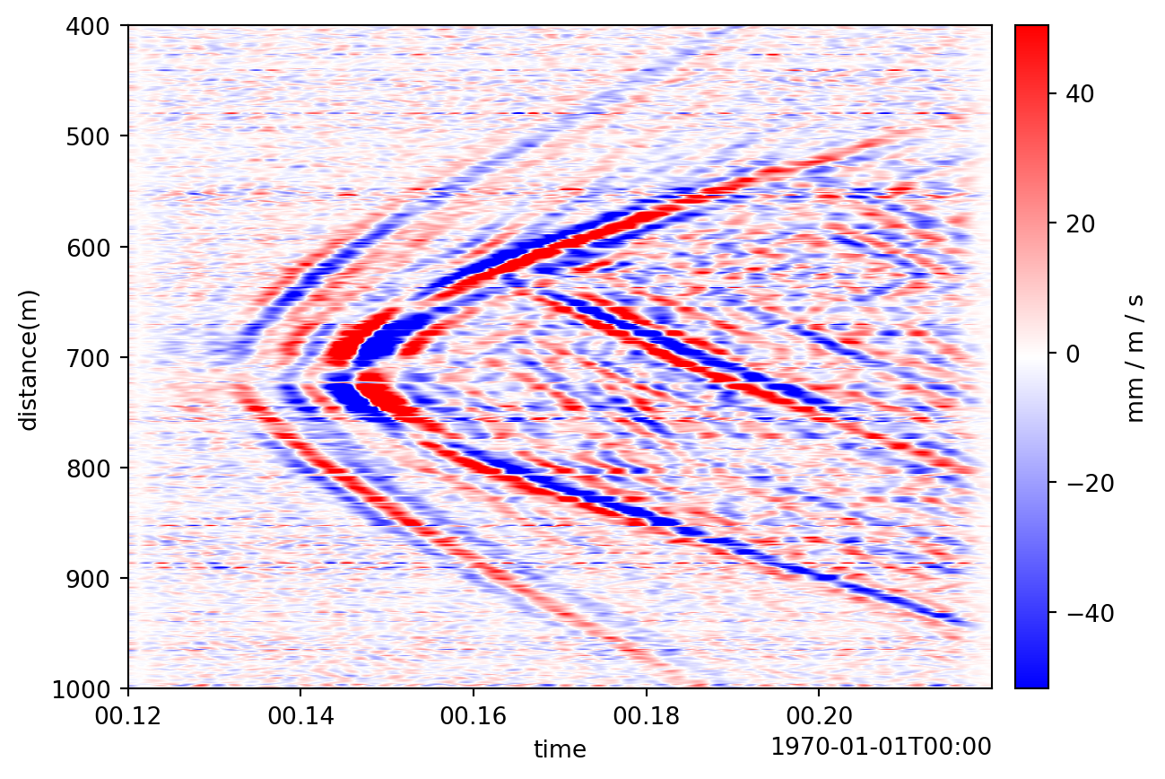
# get example, set unit to velocity (just for demonstration)
patch = dc.get_example_patch().set_units("m/s")

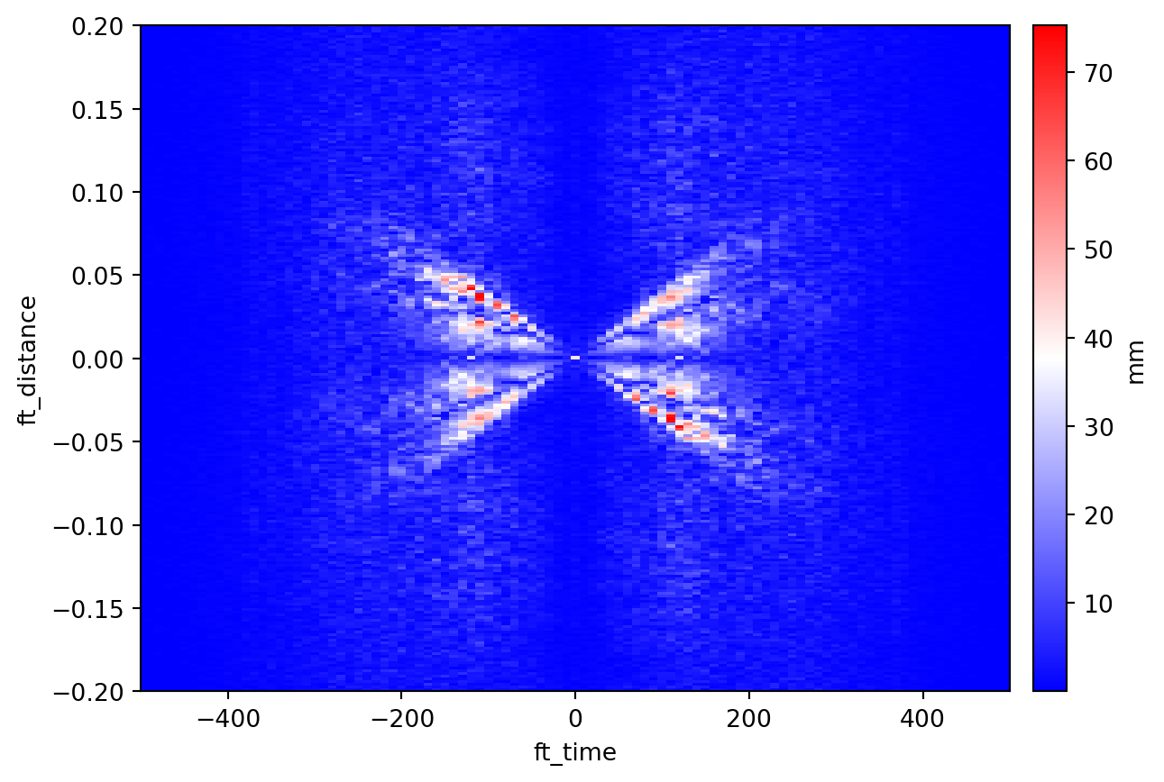
transformed = patch.dft(dim="time")

# note how the dimension name has changed
print(f"old_dims: {patch.dims} new dims: {transformed.dims}")

# as have the units
old_units = patch.attrs.data_units
new_units = transformed.attrs.data_units
print(f"old units: {old_units}, new units: {new_units}")

old_dims: ('distance', 'time') new dims: ('distance', 'ft_time')
old units: 1.0 m / s, new units: 1 m

Note

The transformed dimension names change; “time” becomes “ft_time” indicating the domain of the dimension has changed. The units are also updated. See the note on Fourier transforms in DASCore for more details.

In many cases, it is advantages to only calculate the fourier transform corresponding to the positive frequencies (since the Fourier transform of a real signal is symmetric).

# Transform distance axis to Fourier domain using real fourier transform
real_transform = patch.dft(dim='distance', real=True)
print(real_transform.get_coord("ft_distance"))

CoordRange( min: 0.0 max: 0.5 step: 0.00333 shape: (151,) dtype: float64 units: 1 / m )

The Inverse Discrete Fourier Transform idft undoes the transformation.

# transform back to time domain, take only real component.
patch_2 = transformed.idft().real()
assert np.allclose(patch_2.data, patch.data)

F-k Transforms

F-k transforms are common in geophysics for various types of filtering.

Going back to our example event:

import dascore as dc

patch = (
    dc.get_example_patch('example_event_1')
    .set_units("mm/(m*s)", distance='m', time='s')
    .taper(time=0.05)
    .pass_filter(time=(None, 300))
)

patch.viz.waterfall(show=True, scale=0.2);

We can transform and visualize it in the F-k domain using the dft.

# Apply transform on all dimensions
fk_patch = patch.dft(patch.dims)

# We can't plot complex arrays so only plot amplitude
ax = fk_patch.abs().viz.waterfall()

# zoom in around interesting frequencies
ax.set_xlim(-500, 500);
ax.set_ylim(-.2, .2);